GROMACS tutorial 1: Water
In this introductory tutorial, I'll show you how to create a box of water and run a simple simulation on it with constant temperature and pressure. In the end, we'll find out the density of water.
Setup
Every GROMACS simulations needs three essential files: structure (.gro/.pdb), topology (.top), and parameters (.mdp). The structure file contains the Cartesian coordinates of every atomic site in the system. The topology file contains information on how each atomic site interacts with other atomic sites, whether that is in non-bonded interactions or bonded interactions. This information is provided by the force field. Non-bonded interactions included van der Waals interactions and Coulomb interactions. Bonded interactions include bonds, angles, and dihedrals. The parameters file includes information on how long to run the simulation, the timestep, temperature and pressure coupling, etc. Below we'll obtain/create these files.
At this point, I would suggest creating a directory to store files for this tutorial.
Topology file
We'll start with the topology file. Typically a topology file uses an #include statement to include the force field to be used. This force field includes [ atomtypes ], [ bondtypes ], [ angletypes ], and [ dihedraltypes ] directives. Then in the topology file we usually specify different [ moleculetype ] directives which contain [ atoms ], [ bonds ], and [ dihedrals ] which refer back to the force field. Don't worry about this too much right now. Water models include all of these for us. See Chapter 5 of the reference manual for more information.
Create a file named topol.top with the following text:
#include "oplsaa.ff/forcefield.itp"
#include "oplsaa.ff/tip4pew.itp"

[ System ]
TIP4PEW

[ Molecules ]
As you can see we've included the force field for OPLS-AA. Additionally, we've included the TIP4PEW water model. After this, you'll see a [ System ] directive, which includes just the name of the system, which can be anything you want. Lastly, we list out each moleculetype and how many there are under [ Molecules ]. Right now we don't have any (we'll get those in a minute).
Structure file
The structure of TIP4PEW is already provided by GROMACS in the topology directory. This standard location is typically /usr/share/gromacs/top, but you may have it installed in a different directory. If you are properly sourcing GMXRC then it will be located at $GMXDATA/top. In that directory, you'll see several .gro files, one of which is tip4p.gro. You'll also see the folder oplsaa.ff which we've included in our topology file above. There isn't a structure file specific to TIP4PEW. The four-point water structure is essentially the same for TIP4P and TIP4PEW. What makes them different is the force field parameters.
To create a box of water using that structure file do:
$ gmx solvate -cs tip4p -o conf.gro -box 2.3 2.3 2.3 -p topol.top
If you open back up topol.top you'll see that a line has been added at the end with the word SOL and number. SOL is the name of the moleculetype that is defined in oplsaa.ff/tip4pew.itp. When we ran gmx solvate, GROMACS added enough water molecules to fill a box 2.3 nm in each direction.
Parameter files
Now we need a set of parameter files so that GROMACS knows what to do with our starting structure. Simulations almost always have three main parts: minimization, equilibration, and production. Minimization and equilibration can be broken down into multiple steps. Each of these needs its own parameters file. In this case, we'll be doing two minimizations, two equilibrations, and one production run.
The files we'll be using should be downloaded from here.
There will be a few things common to all five of our files. In each description, I only give a very small comment. See the GROMACS page on this for more information on each option.
| parameter | value | explanation |
|---|---|---|
cutoff-scheme | Verlet | Use in creating neighbor lists. This is now the default, but we provide it here in order to avoid any notes. |
coulombtype | PME | Use Particle-Mesh Ewald for long-range (k-space) electrostatics. |
rcoulomb | 1.0 | Cut-off for real/k-space for PME (nm). |
vdwtype | Cut-off | van der Walls forces cut-off at rvdw. |
rvdw | 1.0 | Cut-off for VDW (nm). |
DispCorr | EnerPress | Long-range correction for VDW for both energy and pressure. |
Cut-off distances should be set keeping in mind how the force field was parameterized. In other words, it's a good idea to look at the journal article that describes how the force field was created. We've chosen 1.0 nm for our cut-offs here, which is common enough for OPLS, but you may determine for your system to choose something else.
Additionally in each part, we'll also be outputting an energy file, a log file, and a compressed trajectory file. The rate of output (in simulation steps) for these is set using nstenergy, nstlog, and nstxout-compressed, respectively. We'll output more information in the production run.
For each part, except for the second minimization, we'll also be constraining all bonds involving hydrogen using the LINCS algorithm by setting constraint-algorithm = lincs and constraints = h-bonds. This allows us to use a larger time step than otherwise.
For the first minimization, we use the steepest descents algorithm by setting integrator = steep to minimize the energy of the system with a maximum of 1,000 steps (nsteps = 1000). The minimization will stop if the energy converges before then. Additionally, we have define = -DFLEXIBLE. This lets GROMACS know to use flexible water since by default all water models are rigid using an algorithm called SETTLE. In the water model's topology file, which we have included, there is an if statement that looks for the FLEXIBLE variable to be defined. The purpose of this first minimization is to get the molecules in a good starting position so we can turn on SETTLE without any errors.
In the second minimization we are simply removing define = -DFLEXIBLE and increasing the number of maximum steps to 50,000.
The last three parts -- the two equilibrations and production -- all use the leap-frog integrator by setting integrator = md. Additionally, each one will use a 2 fs time step by setting dt = 0.002.
For the first equilibration step, there are a few things to note. We are adding several parameters that are shown below:
| parameter | value | explanation |
|---|---|---|
gen-vel | yes | Generate velocities for each atomic site according to a Maxwell-Boltzmann distribution. Only generate velocities for your first equilibration step. This gets us close to the temperature at which we will couple the system. |
gen-temp | 298.15 | Temperature in K to use for gen-vel. Unless you are doing some strange/interesting stuff, this should be the same as ref-t. |
tcoupl | Nose-Hoover | The algorithm to use for temperature coupling. Nose-Hoover correctly produces the canonical ensemble. |
tc-grps | System | Which groups should be temperature-coupled. You can couple different groups of atoms separately, but we'll just couple the whole system. |
tau-t | 2.0 | Time constant for coupling. See the manual for details. |
ref-t | 298.15 | The temperature in K at which to couple. |
nhchainlength | 1 | Leap-frog integrator only supports 1, but by default, this is 10. This is set so GROMACS doesn't complain to us. |
The point of this first equilibration is to get us to the correct temperature (298.15 K) before adding pressure coupling. Adding temperature and pressure coupling at the same time can cause your system to be unstable and crash. We don't want to shock our system at the beginning. Additionally, we have set nsteps = 50000, so with a 2 fs time step, that means that this will run for 100 ps. This is adequate for what we are doing here, but in larger / more complicated systems you may need to equilibrate longer.
The second equilibration adds pressure coupling. Note that we are not generating velocities again, since that will undo some of the work we just did. We also set continuation = yes for the constraints, since we are continuing the simulation from the first equilibration. This part will run for 1 ns. Again, this may need to be longer for other systems.
| parameter | value | explanation |
|---|---|---|
pcoupl | Parrinello-Rahman | The algorithm to use for pressure coupling. Parrinello-Rahman correctly produces the isobaric-isothermal ensemble when used with Nose-Hoover. |
tau-p | 2.0 | Time constant for pressure coupling. See the manual for details. |
ref-p | 1.0 | The pressure in bars at which to pressure couple. |
compressibility | 4.46e-5 | The compressibility of the system in bar^-1. |
For the production run, everything is exactly the same as the last equilibration, except we are outputting more data and running for 10 ns.
Simulation
We have all the files we need now to run each part of the simulation. In each part you typically run gmx grompp to preprocess the three files we now have (.gro, .top, and .mdp) into a .tpr file (sometimes confusingly also called a topology file).
Minmizations
First, let's run our two minimization steps by doing the following:
$ gmx grompp -f mdp/min.mdp -o min.tpr -pp min.top -po min.mdp
$ gmx mdrun -s min.tpr -o min.trr -x min.xtc -c min.gro -e min.edr -g min.log

$ gmx grompp -f mdp/min2.mdp -o min2.tpr -pp min2.top -po min2.mdp -c min.gro
$ gmx mdrun -s min2.tpr -o min2.trr -x min2.xtc -c min2.gro -e min2.edr -g min2.log
At each part, we are reading in the .mdp file with the -f flag. By default if -c and -p flags are not specified GROMACS uses conf.gro and topol.top for the structure and topology files. Additionally we are outputting a processed topology file -pp and mdp file -po. These are optional, but probably worth looking at, especially the processed mdp file, since it is commented.
At each subsequent step we read in the previous step's last structure file or checkpoint file using the -c and -t flags. By default GROMACS outputs checkpoint files every 15 minutes and at the last step. If the checkpoint file is not present, GROMACS will use the structure file defined by -c, so it is a good practice to specify both. At each gmx mdrun we are telling GROMACS to use a default name for each input and output file, since several files are output.
Note we are using -maxwarn 1 for the second minimization. Only use this flag if you know what you are doing! In this case we get a warning about the efficiency of L-BFGS which we can safely bypass.
To get a feel for what's going on, let's extract the potential energy of both of these parts using the GROMACS command gmx energy. Do the following and enter the number that corresponds with Potential, followed by enter again:
$ gmx energy -f min.edr -o min-energy.xvg
Now do the same for the second minimization:
$ gmx energy -f min2.edr -o min2-energy.xvg
The header of the resulting .xvg. file will contain information for use with the Grace plotting program. I use gnuplot so some of these lines will cause errors. I just simply replace every @ character with # in the .xvg. file and then I can use gnuplot. To plot with first start gnuplot:
$ gnuplot
Then in the gnuplot terminal do:
> plot 'min-energy.xvg' w l
To plot the second minimization step do:
> plot 'min2-energy.xvg' w l
Your first plot should look something like this:
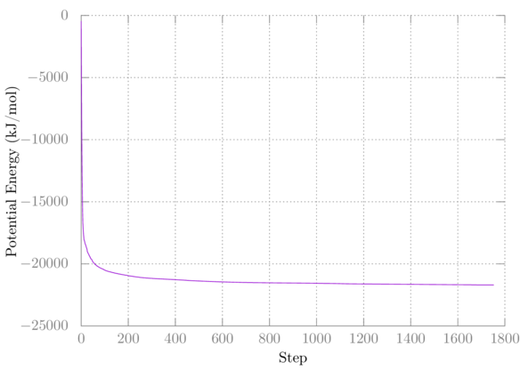
My second minimization didn't change anything, so I have nothing to plot.
Equilibration 1 (NVT)
Now that we have a good starting structure, let's do the first equilibration step, by adding the temperature coupling:
$ gmx grompp -f mdp/eql.mdp -o eql.tpr -pp eql.top -po eql.mdp -c min2.gro
$ gmx mdrun -s eql.tpr -o eql.trr -x eql.xtc -c eql.gro -e eql.edr -g eql.log
Let's take a look at how the temperature varies throughout the simulation:
$ gmx energy -f eql.edr -o eql-temp.xvg
Choose the number corresponding to Temperature at the prompt and hit enter again. Plot it in gnuplot as above. You should see something like:
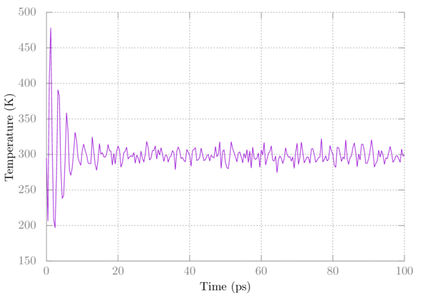
Note that the temperature initially fluctuates wildly but eventually settles.
Equilibration 2 (NPT)
For our last equilibration, as stated earlier, we're adding a pressure coupling:
$ gmx grompp -f mdp/eql2.mdp -o eql2.tpr -pp eql2.top -po eql2.mdp -c eql.gro
$ gmx mdrun -s eql2.tpr -o eql2.trr -x eql2.xtc -c eql2.gro -e eql2.edr -g eql2.log
You can check out the temperature and pressure using gmx energy as above. Here's a plot of the pressure:
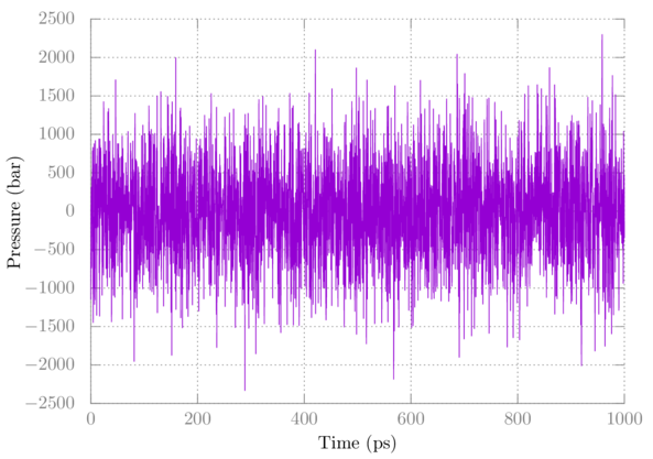
Note that pressure fluctuates quite a bit, which is normal. The average after full equilibration should be close to 1 bar in this case.
Production
Now for the production part do:
$ gmx grompp -f mdp/prd.mdp -o prd.tpr -pp prd.top -po prd.mdp -c eql2.gro
$ gmx mdrun -s prd.tpr -o prd.trr -x prd.xtc -c prd.gro -e prd.edr -g prd.log
Analysis
Using gmx energy as above on prd.edr, get the average temperature, pressure, and density. Are they what you expect?
Here's my output:
Energy                      Average   Err.Est.       RMSD  Tot-Drift
-------------------------------------------------------------------------------
Temperature                 298.145      0.019    8.65629  0.0338992  (K)
Pressure                    3.25876       0.97    688.616   -2.75083  (bar)
Density                     995.381       0.15      12.92  0.0705576  (kg/m^3)
If you look at the TIP4PEW paper in figure 4, you can see we have achieved the correct density. Additionally, note that Wolfram Alpha says the density of water at standard conditions is 997 kg/m^3.
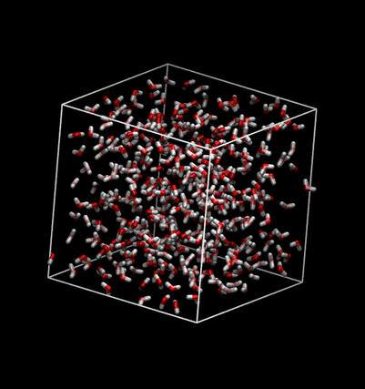
You can also visualize your simulation using a program like vmd. To open the production part with vmd do:
$ vmd prd.gro prd.xtc
Here's a snapshot:
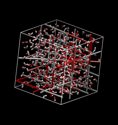
Note that due to the periodic boundary condition this can look kind of strange with bonds stretching across the box. You can make molecules whole by using gmx trjconv:
$ gmx trjconv -f prd.xtc -s prd.tpr -pbc mol -o prd-mol.xtc
Viewing that file should look much nicer:
Summary
In this tutorial, we generate a box of TIP4PEW water using gmx solvate. We simulated it in five distinct parts: minimization 1, minimization 2, equilbiration 1, equilibration 2, and production. Each part used its own .mdp files which were explained. At each part, we used gmx energy to extract useful information about the simulation. After the production run, we were able to find the density of TIP4PEW water.
Author: Wes Barnett, Vedran Miletić