GROMACS tutorial 4: Methane free energy of solvation
In this tutorial, I'll show you how to perform a free energy of solvation simulation using GROMACS, as well as how to calculate the free energy change using MBAR. As always, this tutorial builds off of the previous ones, especially Tutorial 1 and Tutorial 2.
I recommend visiting the Alchemistry website if you are unfamiliar with free energy calculations. This page in particular is relevant. This tutorial follows the direct calculation. State A for us is a methane fully interacting in water. State B will be a methane with all van der Waals and Coulomb interactions with the water turned off; the methane can interact with itself and the water can interact with itself but not with each other. It's as if we have taken the methane out of the water and put it into a vacuum, while somewhere else we still have the water the methane was in. We have 15 total states where we will be linearly turning off the electrostatic interactions and then using a soft-core potential to turn off the van der Waals interactions.
Setup
Box creation
Reuse the methane.pdb and topol.top files that we've been using so far for the OPLS methane and TIP4PEW water. Remove any solvent from the topol.top file (delete the last line which starts with SOL). Make sure that the name for the methane under [ moleculetype ] is 'Methane' (no quotes), as well as under [ molecules ]. We'll be using one methane, so if you have more listed, change it to 1 now.
This time we're using a different box type so that we won't have to use as much water. We'll use a dodecahedron box at 1.2 nm out in each direction from the methane. First, create the box:
$ gmx editconf -f methane.pdb -bt dodec -d 1.2 -o box.gro
Now fill with solvent:
$ gmx solvate -cs tip4p -cp box.gro -o conf.gro -p topol.top
Parameter files
The parameter files we'll be using are almost exactly the same as previous tutorials, except we're adding a free energy section in order to slowly turn off our methane. Additionally, we need a parameter file for each state. We have 15 minimizations, 15 equilibrations, etc. But we'll use a script to simply update the appropriate values in a template, so we actually only will have to have one for each part of the simulation. At each state, we'll do our two minimizations, equilibrate at NVT for 100 ps, equilibrate at NPT for 1 ns, and then do a production run for 5 ns.
The files can be downloaded here.
Here's an explanation of some of these new values:
| parameter | value | explanation |
|---|---|---|
free-energy | yes | Do a free energy simulation. |
init-lambda-state | MYLAMBDA | The value I have in the files is not actually what will be present when we run the simulation. This is a placeholder for an integer number. We are simulating 15 different states, so this number will range from 0 through 14. Our script will replace it for each state. |
calc-lambda-neighbors | -1 | The delta H values will be written for each state. Necessary for MBAR. |
vdw-lambdas | see file | We're turning off VDW at 0.1-lambda increments after electrostatics are off. init-lambda-state=0 corresponds to the first value in this array, init-lambda-state=1 the second, and so on. |
coul-lambdas | see file | We're turning off electrostatics at 0.25-lambda increments first. Just like vdw-lambdas, the init-lambda-state indicates which column is being used. |
couple-moltype | Methane | Matches the name of the [ moleculetype ] in the topology file that we are coupling/decoupling. |
couple-lambda0 | vdw-q | When lambda is 0 (state A) both VDW and electrostatics are completely on. |
couple-lambda1 | none | When lambda is 1 (state B) no nonbonded interations are on. |
couple-intramol | no | Intramolecular terms are not turned off. Usually what you want so you don't have to run it again in vacuum. |
nstdhdl | 100 | How often in steps we're outputting dHdlambda. |
sc-alpha | 0.5 | We're using a soft-core potential for VDW. This parameter is a term in the soft-core function. See the manual. |
sc-power | 1 | See above. |
sc-sigma | 0.3 | See above. |
sc-coul | no | Don't use soft-core for electrostatics. |
One last note on the parameter files: we're using the sd integrator, which stands for stochastic dynamics. sd itself controls the temperature, so we're no longer using Nose-Hoover. If you were to use md you would get a warning that you may not be properly sampling the decoupled state.
Simulation
As stated earlier we're actually running 15 simulations. To make this easier and in order to avoid having 15 different mdp files as inputs, use the following bash script to loop through and run each state:
#!/bin/bash

set -e

for ((i = 0 ; i < 15 ; i++)); do

    sed 's/MYLAMBDA/'$i'/g' mdp/min.mdp > grompp.mdp
    if [[ $i -eq 0 ]]; then
        gmx grompp -o min.$i.tpr -pp min.$i.top -po min.$i.mdp
    else
        gmx grompp -c prd.$(($i-1)).gro -o min.$i.tpr -pp min.$i.top -po min.$i.mdp
    fi
    gmx mdrun -s min.$i.tpr -o min.$i.trr -x min.$i.xtc -c min.$i.gro -e min.$i.edr -g min.$i.log

    sed 's/MYLAMBDA/'$i'/g' mdp/min2.mdp > grompp.mdp
    gmx grompp -o min2.$i.tpr -c min.$i.gro -pp min2.$i.top -po min2.$i.mdp -maxwarn 1
    gmx mdrun -s min2.$i.tpr -o min2.$i.trr -x min2.$i.xtc -c min2.$i.gro -e min2.$i.edr -g min2.$i.log

    sed 's/MYLAMBDA/'$i'/g' mdp/eql.mdp > grompp.mdp
    gmx grompp -o eql.$i.tpr -c min2.$i.gro -pp eql.$i.top -po eql.$i.mdp
    gmx mdrun -s eql.$i.tpr -o eql.$i.trr -x eql.$i.xtc -c eql.$i.gro -e eql.$i.edr -g eql.$i.log

    sed 's/MYLAMBDA/'$i'/g' mdp/eql2.mdp > grompp.mdp
    gmx grompp -o eql2.$i.tpr -c eql.$i.gro -pp eql2.$i.top -po eql2.$i.mdp
    gmx mdrun -s eql2.$i.tpr -o eql2.$i.trr -x eql2.$i.xtc -c eql2.$i.gro -e eql2.$i.edr -g eql2.$i.log

    sed 's/MYLAMBDA/'$i'/g' mdp/prd.mdp > grompp.mdp
    gmx grompp -o prd.$i.tpr -c eql2.$i.gro -pp prd.$i.top -po prd.$i.mdp
    gmx mdrun -s prd.$i.tpr -o prd.$i.trr -x prd.$i.xtc -c prd.$i.gro -e prd.$i.edr -g prd.$i.log

done
The script uses a for loop going from i=0 through i=14. In each iteration it uses sed to find and replace the keyword MYLAMBDA I placed in our mdp file template with the correct lambda state. It saves this file as grompp.mdp which is the default file name that gmx grompp looks for. All of our output is suffixed with the lambda state. Additionally all lambda states greater than 0 use the previous state's final structure file. This isn't entirely necessary for methane decoupling, but it could possibly be beneficial in other systems.
Put the above in a script named run. The script assumes you have downloaded and placed the mdp files in a subdirectory named mdp. Then do:
$ chmod +x run
$ ./run
Analysis
We'll be using MBAR, specifically the python implementation known as pymbar. The alchemical analysis script provides an easy way to perform the calculation and actually provides several different methods with error analysis.
After downloading and installing the script, run it in the directory with the results:
$ alchemical_analysis -p prd. -u kcal
Your output should look something like this:
------------ --------------------- --------------------- --------------------- --------------------- --------------------- ---------------------
    States           TI (kcal/mol)   TI-CUBIC (kcal/mol)       DEXP (kcal/mol)       IEXP (kcal/mol)        BAR (kcal/mol)       MBAR (kcal/mol)
------------ --------------------- --------------------- --------------------- --------------------- --------------------- ---------------------
   0 -- 1         0.002  +-  0.000      0.002  +-  0.000      0.002  +-  0.000      0.001  +-  0.000      0.002  +-  0.000      0.002  +-  0.000
   1 -- 2        -0.000  +-  0.000     -0.000  +-  0.000     -0.001  +-  0.000     -0.000  +-  0.000     -0.000  +-  0.000     -0.001  +-  0.000
   2 -- 3        -0.003  +-  0.000     -0.003  +-  0.000     -0.002  +-  0.000     -0.003  +-  0.000     -0.003  +-  0.000     -0.003  +-  0.000
   3 -- 4        -0.005  +-  0.000     -0.005  +-  0.000     -0.005  +-  0.000     -0.006  +-  0.000     -0.005  +-  0.000     -0.005  +-  0.000
   4 -- 5         0.093  +-  0.002      0.094  +-  0.002      0.090  +-  0.005      0.096  +-  0.003      0.095  +-  0.002      0.094  +-  0.001
   5 -- 6         0.063  +-  0.002      0.065  +-  0.003      0.055  +-  0.010      0.063  +-  0.003      0.064  +-  0.002      0.060  +-  0.001
   6 -- 7         0.013  +-  0.003      0.014  +-  0.003      0.025  +-  0.006      0.009  +-  0.003      0.014  +-  0.003      0.014  +-  0.002
   7 -- 8        -0.055  +-  0.003     -0.052  +-  0.004     -0.051  +-  0.008     -0.050  +-  0.004     -0.052  +-  0.003     -0.052  +-  0.002
   8 -- 9        -0.157  +-  0.004     -0.151  +-  0.005     -0.149  +-  0.014     -0.155  +-  0.006     -0.153  +-  0.004     -0.156  +-  0.003
   9 -- 10       -0.338  +-  0.006     -0.324  +-  0.006     -0.306  +-  0.020     -0.332  +-  0.007     -0.330  +-  0.005     -0.336  +-  0.004
  10 -- 11       -0.602  +-  0.005     -0.621  +-  0.006     -0.595  +-  0.016     -0.631  +-  0.006     -0.626  +-  0.005     -0.627  +-  0.004
  11 -- 12       -0.674  +-  0.003     -0.708  +-  0.003     -0.708  +-  0.005     -0.709  +-  0.004     -0.708  +-  0.003     -0.711  +-  0.002
  12 -- 13       -0.437  +-  0.001     -0.437  +-  0.002     -0.435  +-  0.002     -0.441  +-  0.002     -0.437  +-  0.001     -0.438  +-  0.001
  13 -- 14       -0.138  +-  0.001     -0.134  +-  0.001     -0.131  +-  0.001     -0.132  +-  0.001     -0.131  +-  0.001     -0.130  +-  0.000
------------ --------------------- --------------------- --------------------- --------------------- --------------------- ---------------------
  Coulomb:       -0.007  +-  0.001     -0.007  +-  0.001     -0.006  +-  0.001     -0.007  +-  0.001     -0.007  +-  0.000     -0.007  +-  0.000
  vdWaals:       -2.232  +-  0.015     -2.255  +-  0.015     -2.205  +-  0.033     -2.281  +-  0.013     -2.265  +-  0.010     -2.282  +-  0.013
    TOTAL:       -2.238  +-  0.015     -2.262  +-  0.015     -2.211  +-  0.033     -2.288  +-  0.013     -2.272  +-  0.010     -2.289  +-  0.013
This is the free energy of removing a methane, so the free energy of solvation is actually negative one times this, since it is the reverse process. Our result of 2.289 kcal/mol is comparable to published figures. In a paper that simulated OPLS methane with TIP3P, they achieved a result of 2.44 kcal/mol. The difference can probably be attributed to using a different water model.
Note that the script provides six different results from six different methods. Some of these methods are better than others, but the fact that all six are close to each other tells us we probably sampled enough states to get an accurate number. MBAR is one of the better methods, although BAR and TI are good as well. I reran the script to gather some more analysis:
$ alchemical_analysis -p prd. -u kcal -g -f 20
Here is a visual comparison of the calculated value for each segment:
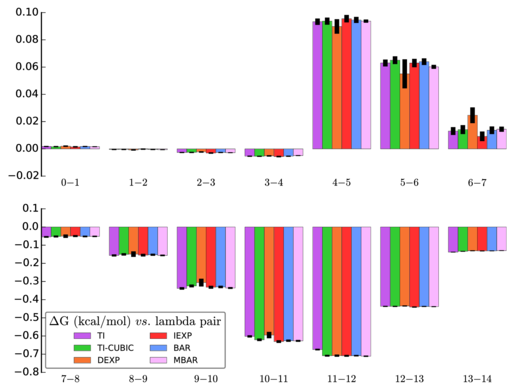
I can see that one of the methods (DEXP) gets different results for calculations between states 5 and 6 as well as between 6 and 7. I'm not too concerned about this, since the other methods line up well and DEXP is not one of the "better" methods.
And here is the <dHdl> curve:
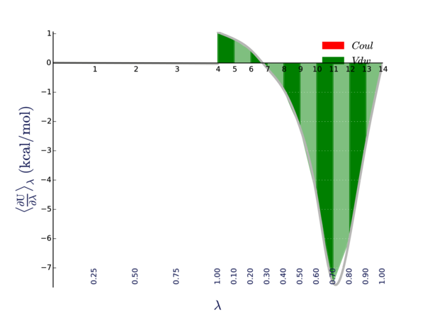
Here we are looking for places where the curvature is high. The curvature is higher around states 10, 11, and 12. Depending on our application, we might want to possibly sample more states in that area.
Lastly, here is a plot of the result calculated as a function of time, both running the simulation forward and running it in reverse:
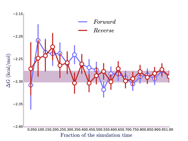
The point here is that we're looking to make sure that the simulation is well-equilibrated; otherwise, the result will not be correct. If the curves were flat for any significant portion of the first part of the plot, this would indicate our system may not be well equilibrated before we started the simulation. We could discard that non-equilibrated data and redo the calculation.
There are a couple of other command-line flags you can use with the alchemical_analysis script. Be sure to check out the homepage of the script and the paper on best practices in free energy analysis which goes much more into detail on these and other plots. I won't go into detail about all the options here.
Summary
In this tutorial, we performed a free energy simulation on methane in water. We turned off electrostatics linearly first, and then we used a soft-core potential to turn off the van der Waals interactions. The intramolecular interactions for methane remained on, so it's as if we were removing the methane from the water and placing it in a vacuum. Our result of 2.289 kcal /mol is comparable to published results.
Author: Wes Barnett, Vedran Miletić